18 Forecasting wildlife habitat (an RSF) with `setupProject`

Author

Eliot McIntire and Julie Turner

Published

June 15, 2026

See Barebones R script for the code shown in this chapter

See the Glossary for definitions of recurring terms (e.g. SpaDES module, dynamic vs. static models, continuous workflow, modular workflow).

Several minutes (<10 minutes) – estimated time for 1st time executing

16 GB RAM (or more) – estimated peak RAM for executing

So far we have combined forest succession (Biomass_core, Biomass_regeneration) with wildfire (scfm) in Forest Succession and Wildfire 17. A common next question is ecological: as the forest grows and burns over the coming decades, how does wildlife habitat change?

In this chapter we answer that for a caribou Resource Selection Function (RSF). An RSF is a fitted statistical model that relates the relative probability of an animal using a location to the covariates at that location (land cover, forest age/biomass, time since fire, etc.). The RSFpredict module takes a previously fitted RSF model and, at each time step, re-evaluates it against the simulated landscape produced by the forest and fire modules. The result is a forecast of habitat selection that responds dynamically to succession and disturbance.

This is a real, three-family project:

forest – Biomass_borealDataPrep, Biomass_core, Biomass_regeneration
fire – the scfm family (scfmDataPrep, scfmIgnition, scfmEscape, scfmSpread, scfmDiagnostics)
wildlife – RSFpredict

Notice that these modules live in different GitHub accounts. Because SpaDES modules declare their inputs and outputs in metadata (see Module Files and Metadata 5), setupProject can weave them into a single coherent workflow even though they were written by different people, at different times, for different purposes.

18.1 The project

The whole project is described by a single setupProject() call. We will show it in full first, then walk through the pieces that are new relative to the forest-and-fire example.

This example pulls its fitted RSF model, study area, and several input layers from Google Drive or other sources.

# get the latest versions of the predictive ecology R packages
repos <- c("https://predictiveecology.r-universe.dev", getOption("repos"))
options(repos = repos)
if (!require("pak")) install.packages("pak")
pak::pak(c("Require", "SpaDES.project"), ask = FALSE)

library(SpaDES.project)

projPath <- "~/SpaDES_book/RSF_forecast"

out <- setupProject(
  # Restart = TRUE, # use this to restart your Rstudio session in its own project
  # useGit = "yourGitHubName",   # optional: clone modules as git repos under your account
  paths = list(projectPath = projPath),
  options = list(
    # We host several files on both GoogleDrive and Compute Canada. This redirects the GoogleDrive
    #   file requests to Compute Canada so we don't need to log in to GoogleDrive
    reproducible.urlRemap =
      "https://object-arbutus.cloud.computecanada.ca/predictiveecology/SCANFI_v2/SCANFI_v2_files_on_arbutus.csv",
    # a shared cloud cache folder, so a whole team can re-use cached results
    reproducible.cloudFolderID =
      "https://drive.google.com/drive/folders/199oEp-TVaCyacwqS4PPf3XWMbhPe4YBN?usp=share_link"
  ),
  modules = c(
    # forest simulation
    "PredictiveEcology/Biomass_borealDataPrep@development",
    "PredictiveEcology/Biomass_core@development",
    "PredictiveEcology/Biomass_regeneration@master",
    # fire simulation -- several modules in one git repository
    file.path("PredictiveEcology/scfm@development/modules",
              c("scfmDataPrep", "scfmIgnition", "scfmEscape",
                "scfmSpread", "scfmDiagnostics")),
    # RSF forecasting
    "JWTurn/RSFpredict@main"
  ),
  params = list(
    .globals = list(
      .plots = "png",
      .studyAreaName = "dehchoN", # Dehcho North in this example
      .useCache = c(".inputObjects", "init"),
      dataYear = 2020,        # start year for predicted forest growth
      sppEquivCol = "LandR"
    ),
    scfmDataPrep = list(
      targetN = 2000,         # keep low for a demo; 4000 is better for real estimates
      .useParallelFireRegimePolys = FALSE,
      .useCloud = TRUE
    ),
    Biomass_borealDataPrep = list(
      .useCloud = TRUE
    ),
    RSFpredict = list(
      simulationProcess = "dynamic"
    )
  ),
  packages = c(
    "httr2",
    "terra", "SpaDES.core (>=3.1.2.9016)",
    "gert", "remotes"
  ),
  times = list(start = 2020, end = 2075),

  # ----- Spatial Templates for our Study -----

  studyArea = reproducible::prepInputs(
    url = "https://drive.google.com/file/d/1ma5qRk2NNidLhrQoiLIzd7W5ogeTaH5-/view?usp=share_link",
    fun = "terra::vect",
    destinationPath = "inputs"),

  # buffer the study area to avoid edge effects in the simulation
  studyArea_biomassParam = terra::buffer(studyArea, 10000),  # -- used in Biomass_borealDataPrep
  studyAreaCalibration = studyArea_biomassParam,             # -- used in scfmDataPrep

  # ----- RSF objects  -----
  # the previously-fitted RSF model object -- used in RSFpredict.R
  model = reproducible::prepInputs(
    url = "https://drive.google.com/file/d/1ILE0WmePubjHiwynSjV_EyetnUhuQIJU/view?usp=share_link",
    fun = "readRDS",
    destinationPath = "inputs"),

  # the land cover the RSF covariates were originally extracted from -- used in RSFpredict.R
  modelLand = reproducible::prepInputs(
    url = "https://drive.google.com/file/d/1LeYrZBKrEPq6jSIP1SWM-grfINTeQjvn/view?usp=share_link",
    fun = "terra::rast",
    destinationPath = "inputs"),

  # ----- raster templates derived from the inputs -----

  # finer than the final RSF resolution, so we can later compute proportions
  rasterToMatch_biomassParam = {
    rtml <- terra::disagg(modelLand[[1]], fact = 2)
    rtml[] <- 1
    terra::mask(rtml, studyArea_biomassParam)
  },
  rasterToMatchCalibration = rasterToMatch_biomassParam,
  rasterToMatch = {
    reproducible::postProcess(rasterToMatch_biomassParam, cropTo = studyArea, maskTo = studyArea)
  },

  # start with the historic fire history so scfm has a realistic time-since-fire
  timeSinceFire = {
    rsts <- reproducible::prepInputs(
      url = "https://drive.google.com/file/d/1D6_Zc-xOttWzTOqasXh6KpGTaXYZ5OMA/view?usp=share_link",
      fun = "terra::rast",
      destinationPath = "inputs")
    tsf <- reproducible::postProcess(rsts$timeSinceFire, to = rasterToMatch)
    tsf <- terra::subst(tsf, 122, NA)   # scfm needs non-forest as NA
    tsf
  }
)

Now run the modules with simInitAndSpades2

results <- SpaDES.core::simInitAndSpades2(out)

18.2 Walking through the new pieces

The structure is the same setupProject() we have used throughout (SpaDES workflows and projects): modules, params, packages, times, and a set of named objects. A few aspects are worth highlighting because they are typical of a real project.

18.2.1 Composing three model families

The modules argument lists modules from two different GitHub accounts (PredictiveEcology, and JWTurn for RSFpredict). The scfm fire model is a family of modules within a single repository, so we build those paths with file.path(). We do not have to tell SpaDES how these fit together – the metadata does that. The forest modules create the initial biomass and age layers from data (currently SCANFI V2.0 for all age, species, biomass layers), scfm creates the initial disturbance layers from SCANFI, and RSFpredict consumes both as its initial inputs. These 3 module families then alternate back and forth through time, feeding each other derived values of these same layers. They are thus, dynamically interacting through forecasted conditions.

18.2.2 `model`: a fitted statistical object as an input

The model object is a previously-fitted RSF (here loaded from an .rds with prepInputs(fun = "readRDS")). This is a good reminder that a SpaDES input can be any R object – not just a map – including a fitted model that a module will apply at every time step. The RSFpredict parameter simulationProcess = "dynamic" tells the module to re-predict against the changing landscape rather than once.

18.2.2.1 Why not fit this RSF here?

To fit an RSF, we need the raw data. For this chapter, we do not have permission to share these data. However, we do have permission to share any RSF models that came from these data (as long as the model doesn’t carry those raw data!). With SpaDES, we can use this approach for now, then replace the model object with a SpaDES module that does the fitting. In fact this is a common approach that we take so that we can refit the statistical model with new data.

18.2.3 Study areas and raster templates

Real projects almost always carry several spatial templates. Here, these are:

studyArea – the area we care about. Here it is a specific, fixed polygon, loaded from a known file and labelled .studyAreaName = "dehchoN". That specificity is what makes cloud caching pay off (see Cloud caching for a team below);
studyArea_biomassParam – a buffered version (here 10 km) so that neighbourhood processes (like fire spread) are not distorted at the edges of the studyArea;
studyAreaCalibration – the area used to calibrate the fire regime (here the same as studyArea_biomassParam).

Each comes with a matching raster template (rasterToMatch, rasterToMatch_biomassParam, rasterToMatchCalibration). Note how these are derived from one another inside the setupProject() call: studyArea is fetched, studyArea_biomassParam is terra::buffer()ed from it, and rasterToMatch is postProcess()ed down from rasterToMatch_biomassParam. Objects defined earlier in the call are available to later ones, so the project description stays in one place.

Building rasterToMatch_biomassParam at a finer resolution (terra::disagg(..., fact = 2)) than the final RSF grid lets the workflow aggregate fine-grained results into proportions later – a common pattern when the response variable is a proportion of a coarser cell.

18.2.4 Cloud caching for a team

Two options here make the cache for expensive data-preparation and fitting steps shareable with: options(reproducible.cloudFolderID = ...) points at a Google Drive folder, and the per-module .useCloud = TRUE parameters (scfmDataPrep, Biomass_borealDataPrep). We don’t need this: the important part of a re-runnable, reproducible, re-usable workflow is that the workflow changes very little or not at all to get these nice behaviours (refit with new data AND use somebody else’s fit if it is already done).

The reason this works is the specific studyArea. Cache decides whether a result can be reused by digesting a function’s inputs (see Introduction to Cache 10); because the study area here is a fixed polygon rather than something randomly generated, every user who runs this project feeds those slow modules the identical inputs, and therefore computes the identical cache key. So once one team member has run the slow scfmDataPrep and Biomass_borealDataPrep fitting and written the result to the shared cloud folder, everyone else downloads that cached result instead of re-running it.

Contrast this with the forest-and-fire example, which builds its study area with LandR::randomStudyArea(): a randomly-drawn area would change the inputs (and the cache key) from user to user, so the cloud cache could not be re-used. Pinning a specific study area is what turns the cloud cache into a genuine team – or workshop or beyond – resource.

18.2.5 `simInitAndSpades2()`

We launch the run with SpaDES.core::simInitAndSpades2(out). The 2 variants of simInit2() / simInitAndSpades2() simply take the list returned by setupProject() directly, instead of having to do.call() it. If the run is interrupted, SpaDES.core::restartSpades() can resume it.

18.3 Examining the finished simulation

Once the run finishes, the same accessors used elsewhere apply.

Code

# generally check out the run

SpaDES.core::completed(results)                       # the events that ran
SpaDES.core::elapsedTime(results, units = "mins")     # time per event

# the forecasted RSF prediction(s) created by RSFpredict
# (object name depends on the module's metadata)
SpaDES.core::moduleMetadata(results)$RSFpredict$outputObjects

18.4 Reporting on datasets used via `prepInputs` (new feature)

If we use prepInputs() to load data, there is a logging feature that keeps a record of the objects we are using (still experimental). This can be very helpful to report on which datasets are being used. As it is experimental (as of reproducible version 3.1.1.9058 and SpaDES.core version 3.1.2.9016), there will be more richness as this grows over time.

Code

reproducible::prepInputsLog() |> data.table::rbindlist()

                      time         fn
                    <char>     <char>
1: 2026-06-15T09:34:27.599 prepInputs
2: 2026-06-15T09:34:31.658 prepInputs
3: 2026-06-15T09:34:33.477 prepInputs
4: 2026-06-15T09:34:34.677 prepInputs
                                                                                     url targetFile archive alsoExtract
                                                                                  <char>     <char>  <char>      <char>
1: https://drive.google.com/file/d/1ma5qRk2NNidLhrQoiLIzd7W5ogeTaH5-/view?usp=share_link       <NA>    <NA>        <NA>
2: https://drive.google.com/file/d/1ILE0WmePubjHiwynSjV_EyetnUhuQIJU/view?usp=share_link       <NA>    <NA>        <NA>
3: https://drive.google.com/file/d/1LeYrZBKrEPq6jSIP1SWM-grfINTeQjvn/view?usp=share_link       <NA>    <NA>        <NA>
4: https://drive.google.com/file/d/1D6_Zc-xOttWzTOqasXh6KpGTaXYZ5OMA/view?usp=share_link       <NA>    <NA>        <NA>
                                  destinationPath cacheId
                                           <char>  <char>
1: /home/emcintir/SpaDES_book/RSF_forecast/inputs    <NA>
2: /home/emcintir/SpaDES_book/RSF_forecast/inputs    <NA>
3: /home/emcintir/SpaDES_book/RSF_forecast/inputs    <NA>
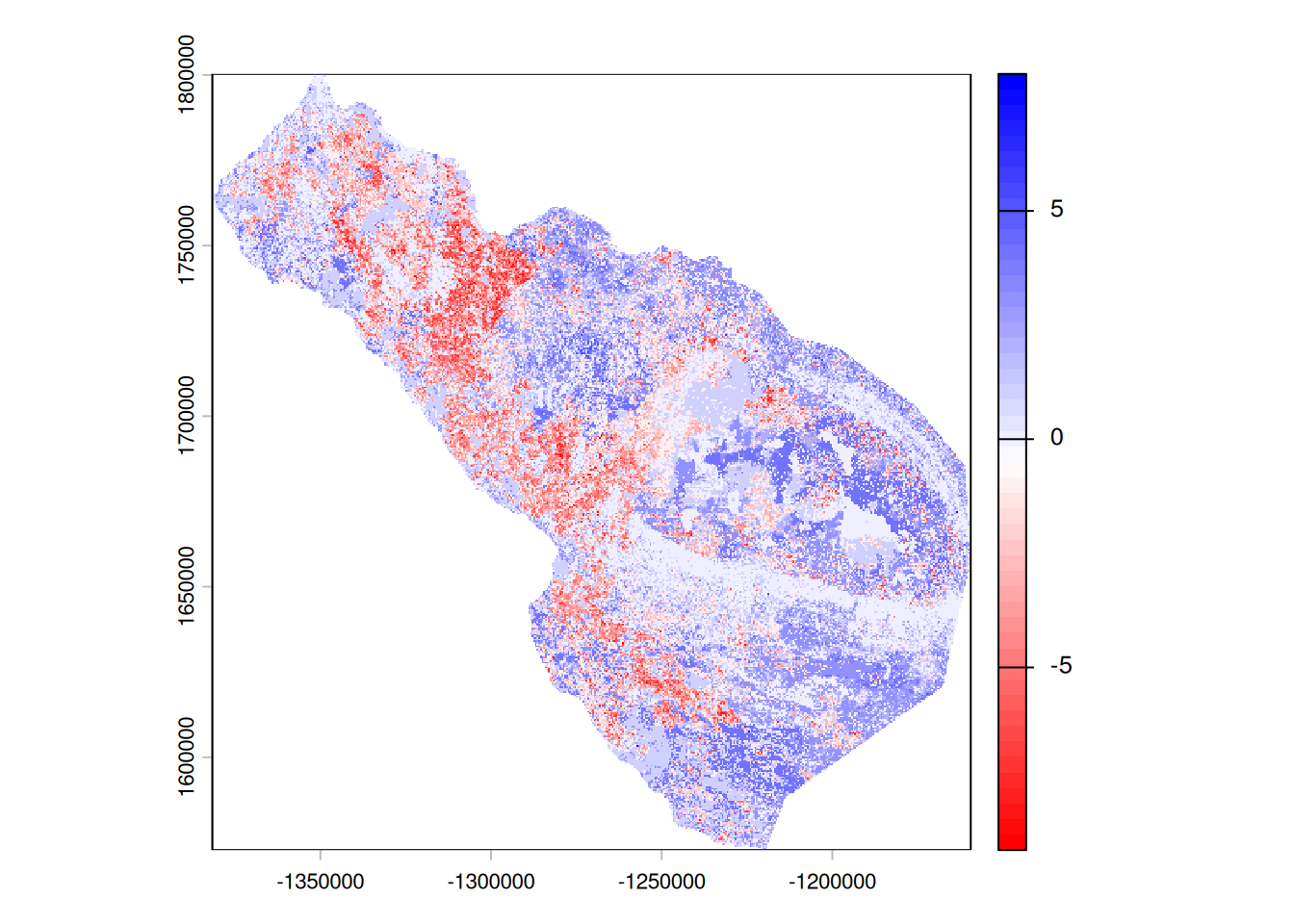
4: /home/emcintir/SpaDES_book/RSF_forecast/inputs    <NA>

Keeping in mind this is one simulation of a simple, toy RSF, we see in general that habitat is worsening between 2025 and 2075 from the absolute predictions simPred, and caribou are predicted to start using the remaining “good” areas more intensely based on the binned maps simBinMap that are relativized yearly. To get at these answers more thoroughly, we would run the simulation many times.

We can look at if the simulated use maps are tending toward better (positive) or worse (negative) habitats for the animals by looking at the differences between the future and current predicted use.

Code

diffMap <- results$simPred$year2075 - results$simPred$year2025
terra::global(diffMap, fun = 'mean', na.rm = T)[[1]]

[1] -0.1020769

Code

diffBinMap <- results$simBinMap$year2075 - results$simBinMap$year2025
terra::global(diffBinMap, fun = 'mean', na.rm = T)[[1]]

[1] 0.1479025

Code

terra::plot(diffBinMap, col = rev(terra::map.pal("differences")))

Difference in RSF predicted bins, 2075 minus 2025

18.5 Using shiny and leaflet to explore outputs

Because we set .plots = "png" and saved maps to the outputPath, the run leaves behind a folder full of time-stamped .tif and .png files – the forecasted forest, fire, and RSF surfaces, one per simulation year. Clicking through those one at a time is tedious. The SpaDES.shiny::shine() function turns that folder into an interactive viewer: it recursively scans the output folder, groups files that share a base name but differ by an embedded timestamp into time-series “objects”, and launches a Shiny app where you can step (or animate) leaflet/leafem (reprojected and tiled so pan/zoom stay fast), while through time. Maps (.tif) are drawn on a choosable web basemap with figures (.png) are shown as images; two extra tabs show the snapshots. You can point it at a simList (it uses that object’s last - first change and a user-defined difference between any two outputPath()), a folder path, or nothing at all (it falls back to getOption("spades.outputPath")).

18.5.1 Using `leaflet`

We can use a tool in SpaDES.project::plotSAsLeaflet() that allows us to automatically show several of the layers using leaflet. If we run it on results, i.e., the simList that exists at year 2075, we will see the state of the rasters and polygons at the end. Since some of them do not change during the 50 years, some will reflect the starting conditions. To know what each object name is, we need to look at the metadata of each module.

Code

SpaDES.project::plotSAsLeaflet(results)

Loading required namespace: leaflet

Loading required namespace: leafem

Warning in x@pntr$writeRaster(opt): GDAL Error 6: plotSAsLeaflet-1.-reproductionMap.tif, band 1: SetColorTable() only
supported for Byte or UInt16 bands in TIFF format.

Warning: [writeRaster] change datatype to INT1U to write the color-table
could not write the color table

Running `postProcessTo`

Running `postProcessTo`
Running `postProcessTo`
Running `postProcessTo`
Running `postProcessTo`
Running `postProcessTo`
Running `postProcessTo`
Running `postProcessTo`
Running `postProcessTo`
Running `postProcessTo`

We can pull out the change over time with:

Code

SpaDES.project::plotChangeOverTime(results)

We can pull out the the time series of each layer that has this with:

Code

SpaDES.project::plotTimeSeriesLeaflet(results)

These functions are intended to be used to explore outputs, rather than present publication-ready visuals.

18.5.2 Using `shiny`

We can get a little more power to visualize with a full shiny web page (but won’t render for this training manual).

Code

if (!require("pak")) install.packages("pak")
pak::pak("SpaDES.shiny")

# explore the saved outputs interactively
SpaDES.shiny::shine("outputs")     # a folder path
# SpaDES.shiny::shine(results)     # or a simList -> uses outputPath(results)

18.6 How is this useful?

Good question! Once we forecast with many iterations, we can estimate habitat change with a level of certainty/uncertainty over all the iterations. The binned maps show where the animals are relatively more or less likely to use than the past, which can help with planning. When linking these modules with others such as fireSense and the LandR.CS suite, we can forecast under different climate change scenarios. More complex models, including human footprint, can be used to predict how cumulative effects may influence space use, aiding in environmental assessments and conservation planning. Current modules in development include simpleHarvest for forest harvests and anthroDistubance in NWT. The possibilities are endless.

18.7 See also

Forest Succession and Wildfire 17

SpaDES workflows and projects

reproducible::prepInputs for Data 12

Introduction to Cache 10

SpaDES.shiny::shine (interactive output viewer)

18.8 Barebones R script

Code

# get the latest versions of the predictive ecology R packages
repos <- c("https://predictiveecology.r-universe.dev", getOption("repos"))
options(repos = repos)
if (!require("pak")) install.packages("pak")
pak::pak(c("Require", "SpaDES.project"), ask = FALSE)

library(SpaDES.project)

projPath <- "~/SpaDES_book/RSF_forecast"

out <- setupProject(
  # Restart = TRUE, # use this to restart your Rstudio session in its own project
  # useGit = "yourGitHubName",   # optional: clone modules as git repos under your account
  paths = list(projectPath = projPath),
  options = list(
    # We host several files on both GoogleDrive and Compute Canada. This redirects the GoogleDrive
    #   file requests to Compute Canada so we don't need to log in to GoogleDrive
    reproducible.urlRemap =
      "https://object-arbutus.cloud.computecanada.ca/predictiveecology/SCANFI_v2/SCANFI_v2_files_on_arbutus.csv",
    # a shared cloud cache folder, so a whole team can re-use cached results
    reproducible.cloudFolderID =
      "https://drive.google.com/drive/folders/199oEp-TVaCyacwqS4PPf3XWMbhPe4YBN?usp=share_link"
  ),
  modules = c(
    # forest simulation
    "PredictiveEcology/Biomass_borealDataPrep@development",
    "PredictiveEcology/Biomass_core@development",
    "PredictiveEcology/Biomass_regeneration@master",
    # fire simulation -- several modules in one git repository
    file.path("PredictiveEcology/scfm@development/modules",
              c("scfmDataPrep", "scfmIgnition", "scfmEscape",
                "scfmSpread", "scfmDiagnostics")),
    # RSF forecasting
    "JWTurn/RSFpredict@main"
  ),
  params = list(
    .globals = list(
      .plots = "png",
      .studyAreaName = "dehchoN", # Dehcho North in this example
      .useCache = c(".inputObjects", "init"),
      dataYear = 2020,        # start year for predicted forest growth
      sppEquivCol = "LandR"
    ),
    scfmDataPrep = list(
      targetN = 2000,         # keep low for a demo; 4000 is better for real estimates
      .useParallelFireRegimePolys = FALSE,
      .useCloud = TRUE
    ),
    Biomass_borealDataPrep = list(
      .useCloud = TRUE
    ),
    RSFpredict = list(
      simulationProcess = "dynamic"
    )
  ),
  packages = c(
    "httr2",
    "terra", "SpaDES.core (>=3.1.2.9016)",
    "gert", "remotes"
  ),
  times = list(start = 2020, end = 2075),

  # ----- Spatial Templates for our Study -----

  studyArea = reproducible::prepInputs(
    url = "https://drive.google.com/file/d/1ma5qRk2NNidLhrQoiLIzd7W5ogeTaH5-/view?usp=share_link",
    fun = "terra::vect",
    destinationPath = "inputs"),

  # buffer the study area to avoid edge effects in the simulation
  studyArea_biomassParam = terra::buffer(studyArea, 10000),  # -- used in Biomass_borealDataPrep
  studyAreaCalibration = studyArea_biomassParam,             # -- used in scfmDataPrep

  # ----- RSF objects  -----
  # the previously-fitted RSF model object -- used in RSFpredict.R
  model = reproducible::prepInputs(
    url = "https://drive.google.com/file/d/1ILE0WmePubjHiwynSjV_EyetnUhuQIJU/view?usp=share_link",
    fun = "readRDS",
    destinationPath = "inputs"),

  # the land cover the RSF covariates were originally extracted from -- used in RSFpredict.R
  modelLand = reproducible::prepInputs(
    url = "https://drive.google.com/file/d/1LeYrZBKrEPq6jSIP1SWM-grfINTeQjvn/view?usp=share_link",
    fun = "terra::rast",
    destinationPath = "inputs"),

  # ----- raster templates derived from the inputs -----

  # finer than the final RSF resolution, so we can later compute proportions
  rasterToMatch_biomassParam = {
    rtml <- terra::disagg(modelLand[[1]], fact = 2)
    rtml[] <- 1
    terra::mask(rtml, studyArea_biomassParam)
  },
  rasterToMatchCalibration = rasterToMatch_biomassParam,
  rasterToMatch = {
    reproducible::postProcess(rasterToMatch_biomassParam, cropTo = studyArea, maskTo = studyArea)
  },

  # start with the historic fire history so scfm has a realistic time-since-fire
  timeSinceFire = {
    rsts <- reproducible::prepInputs(
      url = "https://drive.google.com/file/d/1D6_Zc-xOttWzTOqasXh6KpGTaXYZ5OMA/view?usp=share_link",
      fun = "terra::rast",
      destinationPath = "inputs")
    tsf <- reproducible::postProcess(rsts$timeSinceFire, to = rasterToMatch)
    tsf <- terra::subst(tsf, 122, NA)   # scfm needs non-forest as NA
    tsf
  }
)

# results <- SpaDES.core::simInitAndSpades2(out)



# generally check out the run

SpaDES.core::completed(results)                       # the events that ran
SpaDES.core::elapsedTime(results, units = "mins")     # time per event

# the forecasted RSF prediction(s) created by RSFpredict
# (object name depends on the module's metadata)
SpaDES.core::moduleMetadata(results)$RSFpredict$outputObjects

reproducible::prepInputsLog() |> data.table::rbindlist()

diffMap <- results$simPred$year2075 - results$simPred$year2025
terra::global(diffMap, fun = 'mean', na.rm = T)[[1]]

diffBinMap <- results$simBinMap$year2075 - results$simBinMap$year2025
terra::global(diffBinMap, fun = 'mean', na.rm = T)[[1]]

terra::plot(diffBinMap, col = rev(terra::map.pal("differences")))

SpaDES.project::plotSAsLeaflet(results)

SpaDES.project::plotChangeOverTime(results)

SpaDES.project::plotTimeSeriesLeaflet(results)

# if (!require("pak")) install.packages("pak")
# pak::pak("SpaDES.shiny")
# 
# # explore the saved outputs interactively
# SpaDES.shiny::shine("outputs")     # a folder path
# # SpaDES.shiny::shine(results)     # or a simList -> uses outputPath(results)

18.1 The project

18.2 Walking through the new pieces

18.2.1 Composing three model families

18.2.2 model: a fitted statistical object as an input

18.2.2.1 Why not fit this RSF here?

18.2.3 Study areas and raster templates

18.2.4 Cloud caching for a team

18.2.5 simInitAndSpades2()

18.3 Examining the finished simulation

18.4 Reporting on datasets used via prepInputs (new feature)

18.5 Using shiny and leaflet to explore outputs

18.5.1 Using leaflet

18.5.2 Using shiny

18.6 How is this useful?

18.7 See also

18.8 Barebones R script

18.2.2 `model`: a fitted statistical object as an input

18.2.5 `simInitAndSpades2()`

18.4 Reporting on datasets used via `prepInputs` (new feature)

18.5.1 Using `leaflet`

18.5.2 Using `shiny`